A step-by-step tutorial for building your first data pipeline using Airflow and MLB data

Two-line summary

24 min read

Building a data pipeline - the process of extracting, transforming and surfacing data - is one of the most fundamental skills for a data scientist. In this tutorial, we use Major League Baseball data to incrementally build a simple pipeline in Python via Airflow.

Table of contents

• Reader prerequisites
• What is a data pipeline?
• DAG 101
• Introduction to Airflow
• Setting up your Python environment
• Understanding the data source
• Designing the pipeline
• Building the pipeline skeleton
• Getting data
• Putting it all together
• Closing thoughts

Reader prerequisites

This tutorial assumes that the reader has an elementary understanding of Python, meaning you can import libraries, print statement and write/call simple functions. You will also be required to install packages using the command-line interface (Terminal on Mac) and use a code text editor. I recommend Visual Studio Code or Sublime.

Prior knowledge of data engineering, pipelines and Airflow is not required.

What is a data pipeline?

In the simplest of terms, a data pipeline is a set of tasks that are executed in a particular order to achieve a desired result. Typically, a task is represented by a snippet of code. The order of task execution matters because one task may rely on the outcome of another.

For example, a very simple pipeline would be some code that checks your work calendar and emails you the date and time of your next meeting. In this case we have two tasks: (1) checking the calendar, and (2) sending the email. The email cannot be sent before checking the calendar because it relies on knowing the contents of the upcoming meetings; therefore, we say that the second task is dependent on the first.

Figure 1: An example of a simple data pipeline

Note that how we define the tasks in a pipeline is somewhat arbitrary. We could have, for example, decided to split "check calendar" into two separate tasks: retrieving the meetings data, then filtering them down to the first meeting. The design of the pipeline is left to the discretion of the data engineer and is organized based on efficiency and logical interpretability.

We're using a very simple example here but in practice, most data pipelines have at least three basic functions: fetching data, transforming it and surfacing it to the user. This is otherwise known as an ETL (Extract Transform Load) pipeline.

DAG 101

We can't talk about pipelines without understanding the concept of DAGs, Directed Acyclic Graphs. In fact, the calendar example above is a DAG.

To introduce proper terminology, each task is called a node and the arrow indicating the order of tasks is called an edge. Figure 1 is directed because the edge denotes a fixed order of task execution and it is acyclic because their are no circular dependencies.

If we wanted to make the DAG cyclic, we could update the pipeline so that you could reply "next" to the email and it would recheck the calendar for the next meeting. The new DAG would look something like this:

Figure 2: An example of a cyclic DAG

This graph is cyclic because the email relies on the calendar which relies on the email, and so on. When we write pipelines, it is important that they are acyclic because we have to execute tasks sequentially. Otherwise, there is ambiguity on which task to run first and we reach a deadlock.

Introduction to Airflow

Now that we understand the definition of a pipeline, it is important to understand the role of the components at play. Tasks are snippets of code, which in our case will be written in Python. Airflow is the system that will orchestrate the tasks by defining the structure of the DAG, execute them in the correct order and display results.

Think of Airflow as an air traffic controller and the tasks as flights. Airflow sits at the control centre, dictating when and under what conditions tasks should be run. When we define a DAG in Airflow, it checks each one on a fixed schedule and determines when tasks should be run based on the constraints of the graph.

Following our example from Figure 1, here are the series of checks that Airflow would iterate through in order to complete a single run of the DAG. Yellow indicates a queued task, blue means running and green means completed.

Airflow first checks if either task has a dependency. Since Check calendar does not, it is triggered to run while Send email must wait for its dependency to complete. Airflow rechecks the status of dependencies every few seconds until all tasks are completed, so as soon as Check calendar finishes, Send email is able to be kicked off.

Figure 3: Iterations of tasks triggered by Airflow for a single run of a DAG

Once the DAG has completed running all tasks, Airflow will wait until the next scheduled interval to start the same process again.

Setting up your Python environment

Only install the following if you haven't already. Start by visiting https://brew.sh/ and copying the command under Install Homebrew into Terminal.

Use Homebrew to install Python with the command brew install python3.

Install virtual environment using the command sudo pip3 install virtualenv. A virtual environment allows packages installed in this tutorial to be isolated away from other projects so that we don't create conflicting dependencies. It is not absolutely necessary but it is highly recommended.

Name and activate the virtual environment by running virtualenv -p python venv && source venv/bin/activate. If you've done everything correctly, you should now see a (venv) before your command line.

Now that we're in our virtual environment, we can begin to install packages. Run pip3 install apache-airflow to install Airflow. This will take several minutes. When installation is complete, Airflow needs to be initialized with a user which can be done with the command: airflow db init && airflow users create --username admin --password admin --firstname Anonymous --lastname Admin --role Admin --email admin@example.com.

Finally, we need to install a library that will allow us to request data from external sources. To do this, run the command pip3 install requests.

With that, we're ready to test the Airflow UI! To do this, run airflow webserver. This is a continuous process so you'll want to keep this terminal window open while opening a new one for the next command.

In the new window, make sure you're in the virtual environment (by running virtualenv -p python venv && source venv/bin/activate) and then run airflow scheduler. This is also a continuous process so make sure you keep this window open so that both the webserver and scheduler are running in the background.

Finally, go to your browser and type in localhost:8080. This should take you to your local instance of Airflow. 

Log in with the credentials defined above (username admin, password admin) and you will be taken to a screen of sample DAGs. Et voilà! Your environment is ready to create your first pipeline.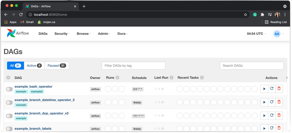

Understanding the data source

The data we use for this pipeline will come from https://appac.github.io/mlb-data-api-docs/. This source does not require user authentication to request data; meaning, it can be accessed freely by anyone with the link. It contains information about baseball players, teams and broadcasted games.

If for some reason this data source is deprecated after this article is published, I've stored sample copies in this folder.

We will use API requests to access the data and for brevity, we won't go through the fundamentals of APIs. It is sufficient to understand that you can tweak URLs to narrow down a specific set of data, which is returned in a hierarchical file format called JSON.

Try it yourself! Visiting this link returns all broadcasted baseball games for the 2021 MLB season: https://lookup-service-prod.mlb.com/json/named.mlb_broadcast_info.bam?sort_by='game_time_et_asc'&season=2021 (may take a few seconds to load). The data appears a bit chaotic but there is a method to the madness. Simply copying and pasting the results into a JSON formatter (many available on google) reveals the underlying structure: there is one entry for each broadcast separated by curly brackets.

As mentioned previously, the power of API requests is that you can tweak the URL to get a different dataset. In fact, everything after the ? in the URL is called a parameter and may be edited to change the request. The parameters are separated by & symbols. Opening the same link but with season=2020 would show the 2020 season, for example.

Figure 4: Unstructured JSON results from broadcast API request

 

Figure 5: Structured JSON results from broadcast API request (same data as Figure 4, put through an online JSON formatter). Each entry is a single broadcast and entries are separated by curly brackets. So, the information about first broadcast is on lines 9-31, the second broadcast on lines 34 and onwards, etc.

Designing the pipeline 

Now that we understand the source, let's lay out the goal for our data pipeline. I'm based out of Toronto, so I'm particularly interested in data around the Toronto Blue Jays. The ultimate goal of the pipeline will be to grab data from the MLB API, filter it down to just Jays data, summarize it and write the results to a file. Specifically, I'd like the file to have all the left-handed players on the current roster as well as the opposing teams for the first ten home games of the 2021 season.

Based on this goal, we're interested in three types of requests:

1. Team data - this link contains one entry per team and maps the name of the team to a team id which we will use to filter steps 2 and 3: http://lookup-service-prod.mlb.com/json/named.team_all_season.bam?sports_code=mlb&season=2021. Again, note that there are two parameters here, the sport and the season have been added at the end of the link to filter the data to only teams that we're interested in. Doing a quick command+F and searching for the Blue Jays shows that the team ID in this entry is 141.

Building the pipeline skeleton

The code for the skeleton of our DAG may be found at this link. Follow along side-by-side as I will reference specific lines that map back to this file.

Lines 1 - 5 import the libraries that we'll need throughout the code. The DAG object will be used to store our DAG structure from Figure 7 and PythonOperator will call the Python code that we write to execute our tasks.

# import necessary libraries
import airflow

from airflow import DAG
from airflow.operators.python import PythonOperator

Lines 7 - 12 declare the DAG object, which I've named mlb_dag. The three fields in the round brackets are mandatory. The dag_id is a name of our choosing and is how the pipeline will appear in the Airflow UI. The start date indicates when the pipeline should start running. This date is arbitrary in our case because there is no scheduled interval, so the pipeline will need to be manually started anyway. We could schedule it to run at regular intervals but for simplicity's sake neither of these fields really matter when the pipeline is unscheduled.

# define DAG
mlb_dag=DAG(
 dag_id="baseball_info",
 start_date=airflow.utils.dates.days_ago(1),
 schedule_interval=None,
)

Now, we need to write Python functions for each of our tasks. For the skeleton, the functions will be left blank; right now they will simply print a statement so that we can test the functionality of the DAG. Later, we will flesh out the code for each task. The tasks are defined on lines 14 - 25 with one function per task to correspond to each node in Figure 7.

Notice that on lines 27 - 50, each function has a corresponding operator. Operators are basically a wrapper around each task that allow Python functions to be callable from your DAG. Using the team task as an example, the operator on lines 28 - 32 (below) will call the function on lines 15 - 16. In the operator, task_id is a human readable name that we'll reference in the DAG structure on line 53, python_callable is the name of the function on lines 15 - 16 and dag is the name of the variable on line 8.

get_team=PythonOperator(
  task_id="get_team",
  python_callable=_get_team,
  dag=mlb_dag,
)

We repeat this code for the other three tasks as well, changing the task id and python callable to match each corresponding function. Finally, we write the structure of the DAG, separating tasks by double arrows. The square brackets indicate a fork, meaning that the get_team task forks into the other two. Note that this must be the last line of your file and that the names should match the task_ids of the four operators.

get_team >> [get_players, get_games] >> write_file

With that, you should have a file matching what is shown in my skeleton file and we are ready to do an initial test of the DAG!

First, create a dags folder inside of your airflow folder by using the command mkdir airflow/dags. Then, copy the skeleton file into this new dags folder using the command cp /{path_to_your_file}/mlb_dag_skeleton.py airflow/dags.

Now open two terminals and run airflow webserver and airflow scheduler the same way we did before (make sure you're in the virtual environment for each one). Navigate to localhost:8080 in your browser and you should be able to see the new DAG listed in the UI. If your DAG has any issues, a red banner will appear at the top of this home screen which you can expand to see error details. 

Click on the DAG name and select "Graph view" from the top of the screen. This will show you exactly the diagram we designed in Figure 7. To run the DAG, flip the toggle on from the left-hand side of the screen and hit the play button on the right side of the screen.

Airflow will now iterate through all tasks, checking dependencies and marking them as complete with the colour-coded green just as we learned with Figure 3 in the Introduction to Airflow section. Each row of these green boxes is a task and each column is a run (we only have one column because we only ran it once). Clicking on an individual box allows you to view the logs from that task.

You can see in the log that the print statement we had for the write_file task is logged here. This means that our operator called the function successfully. 

Now that we know our DAG is functioning, we can start to fill the tasks on lines 15 - 25 with the Python code to actually execute what the tasks are supposed to achieve.

Getting data

In this section, we're going to write the code for the get_team function. All code from this section will be referenced from the final mlb_dag file. Hereafter, all line references will be to this file.

A few housekeeping items: 

1. Now that we're ready to get actual data, we need the requests library. Add import requests as I've done on line 3.
2. Since we used "baseball_info" as the dag_id in the skeleton file, we'll name this one "baseball_info_v2" to avoid confusion. I've made this change on line 10.

Replace the get_team function with the following code (lines 16 - 24 in the final file). Breaking this down line by line, we first store the API request in the response variable (line 18), then grab the JSON portion of the response and access the team entries (line 19). The data is nested within the 'team_all_season', 'queryResults' and 'row' lines, so this line basically extracts the entries from the nested structure of the JSON.

On line 20, I added a line to log the response code from the data source just in case the DAG fails. This will allow us to identify whether it was due to the source being deprecated. If it succeeds, the code will be 200 (full list of codes here). Finally, we use line 23 to filter the teams variable down to only those matching "Toronto Blue Jays". Hypothetically this should only return one entry but since the team variable is a list, I return team[0] so that the function returns an integer.

def _get_team():
  # request team data
  response = requests.get("http://lookup-service-prod.mlb.com/json/named.team_all_season.bam?sports_code='mlb'&season='2021'")
  teams = response.json()['team_all_season']['queryResults']['row']
  print(f"MLB lookup service API response code for team data: {response.status_code}")

  # find blue jays team id
  team = list(x['team_id'] for x in teams if x['name_display_full'] == "Toronto Blue Jays")
  return team[0]

To test, save the file and reload your localhost to see the new DAG.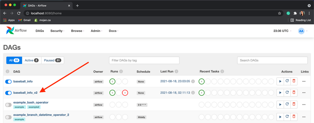

You can see that I attempted this DAG many times, where each column is a run and each task is a row. The rightmost column is the most recent attempt, and you can click on the first row to see the logs for of our new get_team function.

Just as we saw in the first step of the Designing the pipeline section, our function is able to fetch data and filter it down correctly to the Blue Jays team id.

Putting it all together

The remainder of the code involves finishing the get_players, get_games and write_file functions. Line references will be in the same file as the last section, here. Again, a few housekeeping items:

1. These tasks will need to reference the team id from the first task, so we need to grant access to the value returned by it. We do this by adding provide_context=True to each of the three operators on lines 82, 89 and 96. The get_team operator does not need context because it doesn't use values from other tasks.
2. We also need to pass the context to each of these three functions, which we do by adding it as a parameter (**context) on lines 26, 38 and 56.

For the get_players function, we first need to fetch the team id from the first task. We use xcom to do this, copying line 28 from the documentation and replacing the task id with the team function name. This line will store whatever was returned by the get_team function which in our case is a single integer: 141 (Blue Jays team id). The rest of the function is straightforward, noting that we're looking for left-handed players, hence why I filter down to entries with bats attribute equal to 'L' on the last line.

def _get_player(**context):
  # fetch team values from team task
  team_id = context['task_instance'].xcom_pull(task_ids='get_team')

  # get player data from API
  response = requests.get(f"https://lookup-service-prod.mlb.com/json/named.roster_40.bam?team_id='{team_id}'")
  players = response.json()['roster_40']['queryResults']['row']
  print(f"MLB lookup service API response code for players data: {response.status_code}")

  # filter to left-handed batters
  return list(x for x in players if x['bats'] == 'L')

The get_games function is very similar to the last two. The only difference is that the URL does not allow for team_id as a parameter, so we filter the data manually on line 48. The loop iterates through the first ten entires (which are sorted by ascending date as indicated by the URL parameters), storing the away team attribute of each entry.

Finally, the write_file function grabs the results of the players and games on lines 58 - 59. It then loops through each one individually, writing them to the file line-by-line. At long last, the pipeline is complete! Save the file, refresh localhost and trigger a run. If everything works correctly, you should see a file appear on your desktop.

Closing thoughts

Though this tutorial is relatively long for a blog post, it's amazing how transferrable the basics shown here are to industry practice. My last three big tech employers use drastically different data stacks but the fundamentals are the same, and Airflow is a fantastic gateway into data engineering. To learn more about Airflow and its full capabilities, I recommend the book Data Pipelines with Apache Airflow and the Airflow documentation.

As always, would love to hear your thoughts and feedback in the comments below.